0-dimensional geometries, or point geometries, are tied to a single, exact position on the x-y plain. In its most basic form, these geometries are points. Therefore, ggplot2 and Vega-Lite have a point geometry, in Observable Plot this geometry is called a dot. This geometry is mostly used to produce scatter plots.

A scatterplot made in ggplot2 using the point geometry. Source: Maarten Lambrechts, CC BY SA 4.0
Point geometries do not necessarily need to be dots or little circles. Points in ggplot2 and Vega-Lite have a shape aesthetic that can be used to show categorical data.
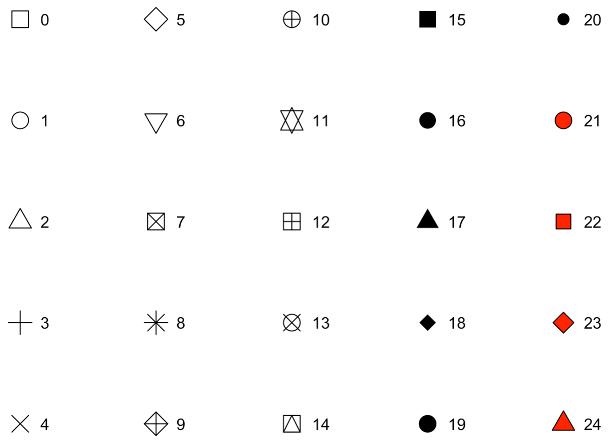
The 24 shapes that can be used for point geometries in ggplot2. Source: Maarten Lambrechts, CC BY SA 4.0, adapted from ggplot2.tidyverse.org/articles/ggplot2-specs.html
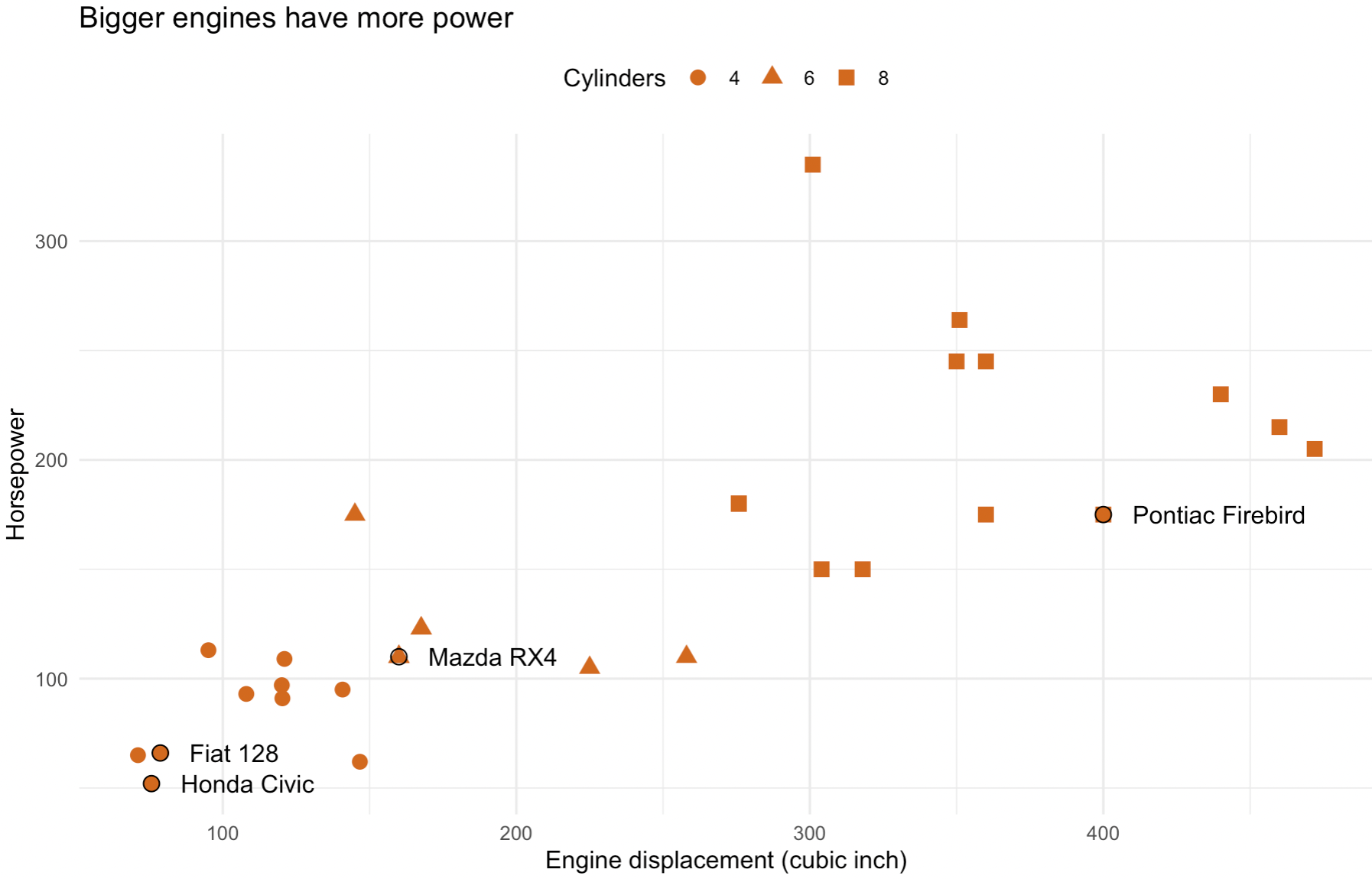
The shapes of the poin geometry in ggplot2 in use. Source: Maarten Lambrechts, CC BY SA 4.0
Vega-Lite has a tick geometry which produces short lines instead of dots or other shapes. It can be used to create very compact visualisations of distributions.

Source: vega.github.io/vega-lite/examples/tick_strip.html
A last type of point geometry is the vector. It uses additional rotate and length aesthetics to produce directed arrows. Observable Plot has a vector geometry, while ggplot2 has a similar spoke geometry.
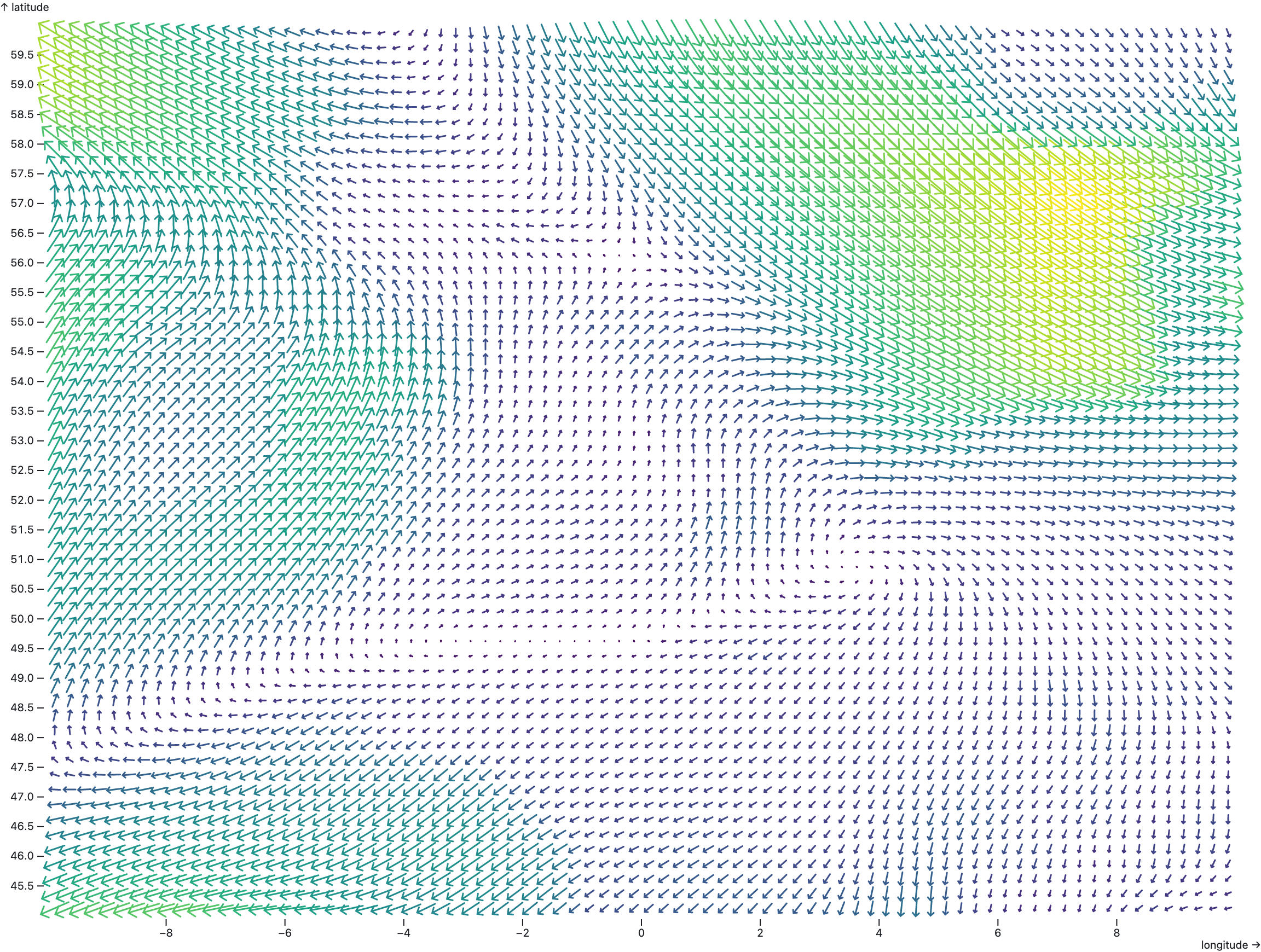
Example of the vector geometry of Observable Plot. Source: observablehq.com/@observablehq/plot-vector
The table below gives an overview of the point geometries and their aesthetics in ggplot2, Vega-Lite and Observable Plot.
| Implementation | Geometry name | Required aesthetics | Additional aesthetics |
|---|---|---|---|
| ggplot2 | geom_point | x, y | shape |
| ggplot2 | geom_spoke | x,y | angle, radius |
| Vega-Lite | point | x, y | shape |
| Vega-Lite | tick | x, y | |
| Observable Plot | dot | x, y | |
| Observable Plot | vector | x, y | rotate, length |